CASE STUDY / CENTRIFUGAL PUMP

Centrifugal pump
CFD analysis.

PyFluent automation, CPU/GPU comparison and steady performance curves, followed by sliding-mesh analysis of pressure pulsation at the volute tongue.

MY CONTRIBUTION

I developed the PyFluent workflow and carried out the steady, transient and spectral analyses.

ANSYS FLUENT 2025 R2 · PYTHON

7 blades · 7000 rpmStartup · 1 revolution in slow motion

2.29×GPU speedup104.0 → 45.45 min · matched 900 L/h run 69.96%Highest simulated MRF efficiency1050 L/h · 10.44 m head 816.67 HzBlade-passing frequencyIdentified in the tongue-pressure spectrum

RELATED PROFESSIONAL WORK / PUMP INTEGRATION

Assess mean performance and pressure pulsation separately.

The engineering question

Integrating a pump changes its inlet and outlet flow paths. Hydraulic performance and the pressure fluctuations generated near the volute tongue both need attention.

My contribution

My professional work combined flow-path studies with transient rotor–stator analysis. I developed Python PSD and pressure-RMS processing when the solver’s built-in analysis was too limited.

This demonstration

The generic pump connects that experience to an automated performance sweep, a CPU/GPU comparison and a sliding-mesh pressure spectrum. Each output answers a different engineering question.

Related professional work covered pump packaging, suction-flow conditioning and hydroacoustics. The curves, timing comparison and spectra on this page belong to the public demonstration; a local pressure spectrum is not a far-field sound prediction.

01 / PYFLUENT AUTOMATION

Automated setup and
operating-point sweeps.

Separate scripts handle model setup, operating-point runs and post-processing. The flow sweep and CPU/GPU comparison use the same saved MRF setup.

PREPARE

Model setup

The setup scripts define the MRF mesh, rotating region, boundary conditions and reports for pressure, flow and torque. The resulting case is reused for each run.

EXECUTE

Batch execution

The sweep reads flow rates from a CSV and launches a separate run for each enabled point. Each run loads the setup, applies the flow rate, initializes, solves, saves and closes Fluent.

CHECK

Result checks

The scripts check report completeness and evaluate the final 200 iterations. Head, torque and efficiency are calculated, and nonstationary points are excluded from the curve fits.

REPEATABLE EXECUTION

Solver configuration

The runner reads the backend, precision, processor count and operating conditions from a configuration dictionary. The sequence keeps each operating point reproducible and its reports comparable.

Workflow summary

Load the configured physical model
Set the operating point and verify reports
Initialize, execute and retain the result for comparison

RUN CHECKS

The GPU runner checks pressure-report averaging, resets histories and waits for asynchronous report output. Previous valid results are kept until the new Fluent session launches successfully.

The transient runner uses the final saved mesh and sampling plan. The recovered SMM meshing script is not a verified CAD-to-mesh workflow.

02 / STEADY MRF PERFORMANCE

Steady pump performance

The MRF flow sweep at 7000 rpm provides head, torque and hydraulic efficiency across the operating range. Five operating points passed the stationarity checks. MRF provides the mean performance map; sliding mesh is used for the pressure-pulsation study.

Mesh: 2.096 million cells
Model: Pressure-based · k–ω GEKO
Fluid properties: $ρ = 1074 kg m^{- 3}$
$μ = 0.004296 Pa·s$
Boundary conditions: Pressure inlet
Mass-flow outlet

Total-pressure head

H = \frac{Δ p_{t}}{ρ g}

Pressure rise expressed as hydraulic head.

Power transfer

P_{hyd} = Q Δ p_{t}

P_{shaft} = | T_{z} | ω

Hydraulic efficiency

η_{h} = \frac{P_{hyd}}{P_{shaft}}

Ratio of useful hydraulic power to impeller input.

$Δ p_{t} = p_{t,out} - p_{t,in}$ , using mass-flow-weighted total pressure. Static-pressure reports use area weighting. Q is in m³/s and $ω = \frac{2 π N}{60}$ . Efficiency describes hydraulic power relative to impeller shaft power; motor and electrical losses are outside this calculation.

FIGURE 01

Head–flow curve

Across the accepted points, head falls from 10.92 m at 900 L/h to 4.25 m at 1650 L/h. A quadratic fit describes this simulated interval with $R^{2} \approx 0.9996$ .

The 450, 600 and 750 L/h cases failed the final stationarity gate. They remain available as diagnostics but are excluded from the performance fit.

Head–flow curve at 7000 rpm. Five accepted points from 900 to 1650 litres per hour show falling head; the highest-efficiency simulated point is marked at 1050 litres per hour. — H–Q curve · five stationary, positive-head points. Full-size figure ↗

FIGURE 02

Efficiency and BEP

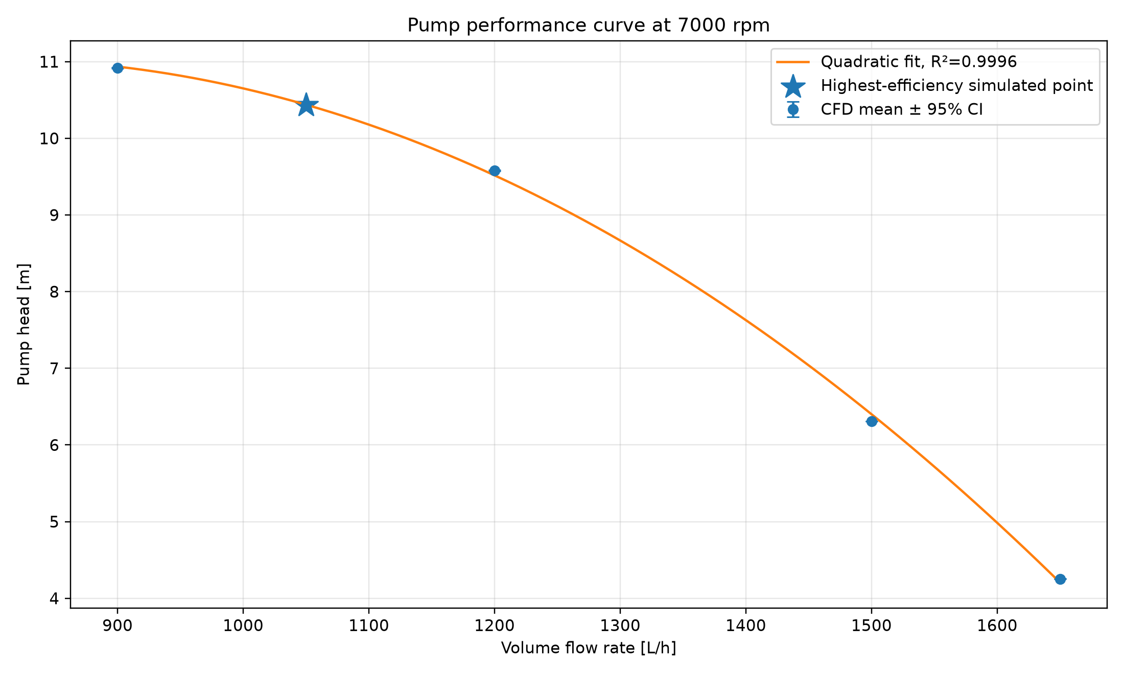
The highest-efficiency simulated point is 1050 L/h, 69.96%, with 10.44 m head. This flow rate sets the operating point for the transient study.

The fitted curve estimates a BEP near 1020 L/h and 70.35%. This point was interpolated, not simulated. The estimate applies to the accepted flow range.

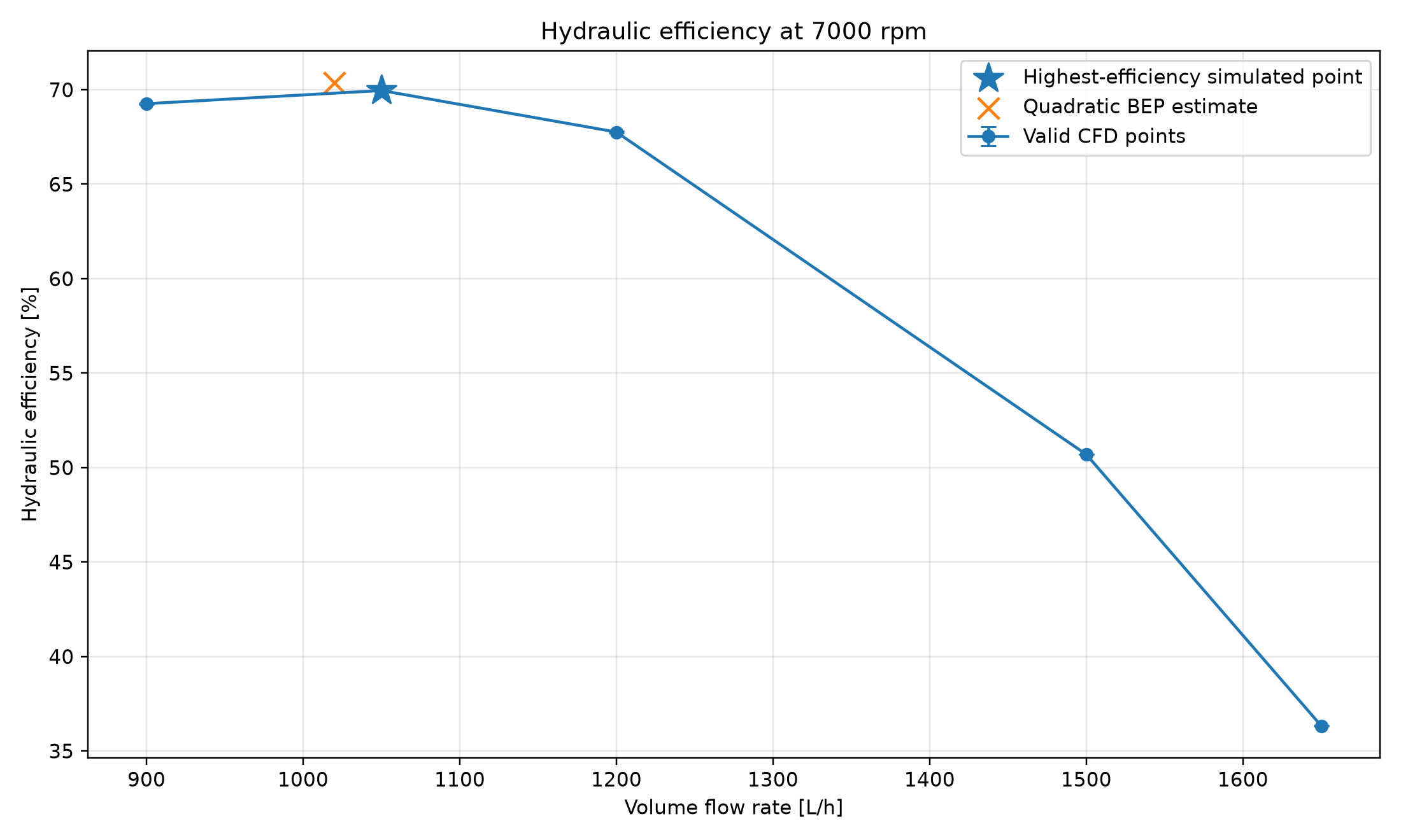
Hydraulic efficiency versus flow, showing a highest simulated efficiency of 69.96 percent at 1050 litres per hour and an interpolated peak of about 70.35 percent near 1020 litres per hour. — Simulated points and fitted best-efficiency estimate are distinguished. Full-size figure ↗

Stationarity checks

The final-window coefficient of variation and fitted drift must meet 1% relative limits, with absolute tolerances for near-zero pressure signals. Accepted points must also have total-pressure rise ≥ 1 kPa and positive shaft power.

The plotted 95% intervals are nominal final-iteration mean intervals $\frac{1.96 s}{\sqrt{n}}$ . They describe numerical history scatter, not mesh, turbulence-model or experimental uncertainty; iteration correlation can make them optimistic.

Accepted MRF points · 7000 rpm
Target Q [L/h]	Head [m]	$η_{h}$ [%]
900	10.919	69.259
1050	10.435	69.956
1200	9.580	67.759
1500	6.310	50.693
1650	4.254	36.329

Download full sweep summary ↓

03 / CPU vs NATIVE GPU

GPU runs took
56.3% less time.

The CPU and Native GPU comparison uses the same 2.096-million-cell setup at 900 L/h and 7000 rpm. Both runs used 1000 iterations, with statistics calculated over the final 200.

CPU · 14 cores104.00 min

Fluent Native GPU45.45 min

58.55 min saved in this matched run

These are calculation wall times for this case; preprocessing and post-processing are outside the comparison.

Speedup

\frac{6240}{2727} \approx 2.29 \times

Wall-time reduction

(1 - \frac{2727}{6240}) \times 100 % \approx 56.3 %

Engineering agreement · GPU relative to CPU
Quantity	CPU	GPU	Δ [%]
Flow [L/h]	899.974	899.956	−0.002
$Δ p_{t}$ [kPa]	114.244	115.068	+0.722
Head [m]	10.8469	10.9252	+0.722
\|Torque\| [N·m]	0.057121	0.056623	−0.870
$η_{h}$ [%]	68.209	69.303	+1.604

Efficiency differs by 1.094 percentage points, equivalent to 1.604% relative to the CPU value.

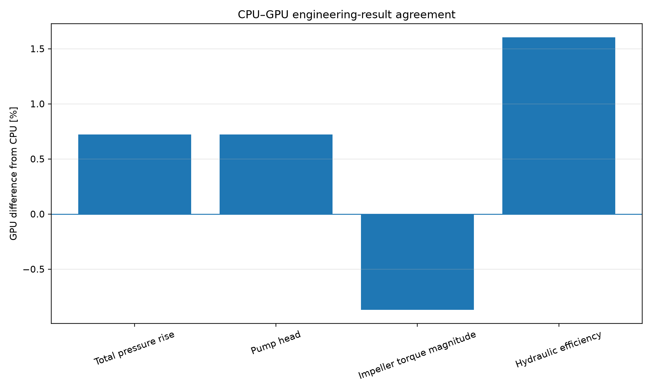
Relative differences between the Native GPU and CPU results, including approximately 0.72 percent in head, minus 0.87 percent in torque and 1.60 percent in hydraulic efficiency. — Relative CPU/GPU differences in stationary mean results. Full-size figure ↗

COMPARISON SCOPE

The GPU run reduced calculation time with a 0.72% head difference and a 1.60% relative efficiency difference. This comparison covers one operating point and does not establish experimental accuracy. The recorded hardware information specifies 14 CPU cores; the GPU model is not documented.

The dedicated 900 L/h repeat is kept separate from the original H–Q sweep snapshot, so its values are not substituted into that curve. Agreement data ↓ · Timing data ↓

04 / TRANSIENT SLIDING MESH

Transient model
and time step

The sliding-mesh model at 1050 L/h and 7000 rpm resolves pressure changes as the seven impeller blades pass the volute tongue. The rotor physically moves across non-conformal interfaces.

The transient mesh contains approximately 2.48 million cells, with separate rotor, casing and pipe regions. The tongue is the stationary volute feature near the discharge where the passing blade flow interacts with the casing. An area-averaged static-pressure monitor on wall_tongue captures its local unsteady loading.

Sliding-mesh startup · 1.5 revolutionsShown in slow motion. Pressure statistics use a separate post-warm-up record.

01 · Rotation

f_{rot} = \frac{N}{60} = \frac{7000}{60}

116.6667Hz

One revolution takes 8.5714 ms.

02 · Blade passage

f_{BPF} = Z f_{rot} = 7 f_{rot}

816.6667Hz

Seven blade passages per revolution.

03 · Time resolution

N_{step/rev} = 7 \times 20

140steps / rev

20 samples per blade passage.

Physical time step

Δ t = \frac{1}{f_{rot} N_{step/rev}}

= \frac{60}{7000 \times 140} s

STEP SIZE61.2245 μs

140 steps per revolution

Warm-up and sampling

10 revWarm-up · 1400 steps

20 revSample · 2800 steps

Discard 85.714 ms of warm-up and retain the next 171.429 ms: 30 revolutions and 4200 steps in total. The plan permits up to 15 inner iterations per time step.

Blade-passage sampling is the basis for this Δt. Establishing temporal accuracy additionally requires time-step refinement and convergence checks within each step; the sampling plan alone does not demonstrate either.

Sampling frequency $f_{s} = \frac{1}{Δ t}$: 16.333 kHz
Nyquist frequency $f_{Nyquist} = \frac{f_{s}}{2}$: 8.167 kHz
Record bin spacing $Δ f = \frac{1}{T}$: 5.833 Hz
BPF location in the full-record FFT: Bin 140
Blade passages in the sampled record: 140

An integer number of revolutions aligns the ideal BPF with a Fourier bin. The Hann window still addresses leakage from other content. Bin spacing is not the same as the window’s ability to resolve nearby peaks; Nyquist is a sampling limit, not a validated accuracy range.

SAMPLED OPERATING POINT

1049.84 L/h

11.00 m head

71.85% hydraulic efficiency

Mean operating point

Between the first and second 10-revolution halves, head changes by about 0.14%, torque by 0.04% and efficiency by 0.18%. This supports using the full record for mean performance. Local pressure amplitudes still evolve, so stable global means do not establish a stationary spectrum.

Transient efficiency uses mean powers: 33.78 W hydraulic / 47.02 W shaft. MRF and SMM use different meshes and formulations; their efficiency difference cannot be attributed solely to unsteadiness.

05 / TONGUE PRESSURE

Tongue-pressure history

Fluent records the area-averaged static pressure on the tongue wall at each time step. The 2800 post-warm-up samples provide the mean pressure, fluctuations and spectra.

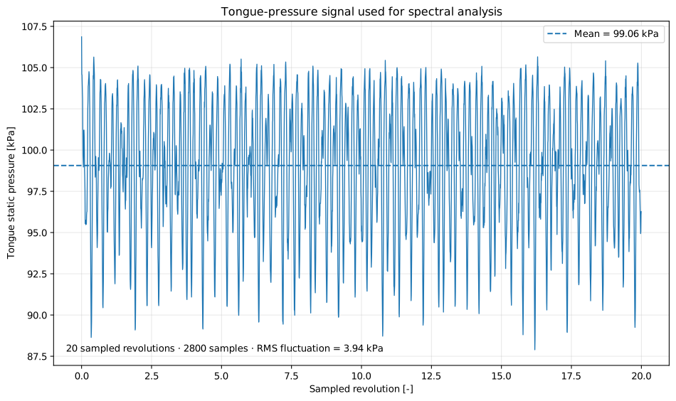
Area-averaged static pressure on the volute tongue over 20 sampled revolutions. The fluctuating trace surrounds a mean of 99.06 kilopascals. — Area-averaged tongue pressure over 20 sampled revolutions. Revolution zero marks the start of sampling, after warm-up. Full-size figure ↗

Spatial average · each step

p_{A} (t) = \frac{1}{A} \int_{A} p (x, t) d A

One pressure value over the tongue surface at each time step.

Temporal mean · 2800 samples

\bar{p} = \frac{1}{n} \sum_{i = 1}^{n} p_{A, i}

99.064kPa

The baseline over the complete sampled record.

Mean-removed fluctuation

p_{i}^{'} = p_{A, i} - \bar{p}

This fluctuation sequence is the input to the pressure spectrum.

RMS pressure fluctuation

{p^{'}}_{RMS} = \sqrt{\frac{1}{n} \sum_{i = 1}^{n} {(p_{i}^{'})}^{2}}

3.938kPa

Overall fluctuation magnitude across the accepted record.

Revolutions → elapsed time

t_{sample} = \frac{n_{rev}}{f_{rot}}

0.171429s

20 sampled revolutions at 116.6667 Hz.

The scalar mean establishes the pressure baseline. The PSD is computed from the sequence of fluctuations $p^{'} (t)$ over the 2800-sample record.

PRESSURE POST-PROCESSING

The postprocessor joins the performance and tongue-pressure reports by time step and calculates elapsed time using the saved sampling plan. Subtracting the temporal mean removes the DC component before spectral analysis.

06 / PRESSURE SPECTRUM

Pressure spectrum and
blade-passing frequency

The PSD and RMS amplitude spectrum quantify the frequency content of the pressure fluctuations. Comparisons across sampling windows and individual revolutions assess the stability and phase consistency of the main components.

FIGURE 05

Pressure PSD

The one-sided spectral density has units of Pa²/Hz. Integrating a frequency band gives its estimated pressure variance; its square root gives band RMS. A PSD peak height by itself is not a harmonic RMS amplitude.

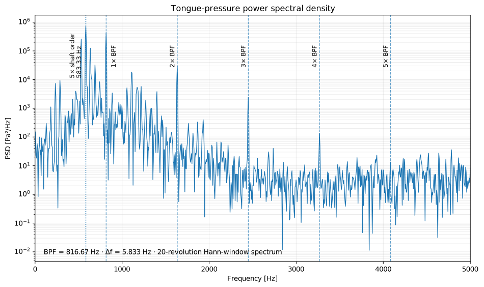
The postprocessor calls SciPy’s Welch routine with density scaling and no additional detrending after mean removal. Its full-record default uses all 2800 samples in one Hann segment, so it reduces to a modified periodogram rather than an average over multiple independent segments. The displayed record has 5.833 Hz bin spacing; shorter Welch segments would trade frequency resolution for averaging.

FIGURE 06

RMS amplitude spectrum

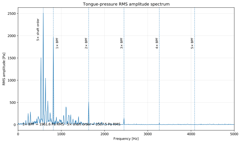
The one-sided FFT is corrected for Hann-window coherent gain and converted from peak to RMS amplitude for the interior positive-frequency bins. This makes the blade-passing components interpretable in pressure units.

RMS pressure amplitude spectrum: fifth shaft order at 583.33 Hz is about 2507.5 Pa RMS, exceeding the BPF amplitude of 1961.6 Pa RMS at 816.67 Hz. — RMS line amplitudes · the fifth shaft-order peak exceeds the BPF in the full pressure record. Full-size figure ↗

Tongue-pressure BPF harmonics
Harmonic	Frequency [Hz]	RMS [Pa]
1× BPF	816.67	1961.6
2× BPF	1633.33	508.7
3× BPF	2450.00	147.2
4× BPF	3266.67	34.3
5× BPF	4083.33	10.9

Fifth shaft-order component

The BPF fundamental leads its harmonic family, with rapidly decreasing amplitudes at higher orders. However, the full pressure spectrum contains a stronger component at $583.33 Hz = 5 f_{rot}$ : approximately 2507.5 Pa RMS, versus 1961.6 Pa RMS at the BPF.

The 5×/BPF amplitude ratio changes from about 0.96 in the first 10 revolutions to 1.45 in the last 10. It is about 1.28 over the full record, so the fifth-order component remains significant in both the full and later sampling windows.

PHASE ANALYSIS

Phase consistency across revolutions

Per-revolution complex harmonic analysis shows strong phase consistency at the BPF in both tongue pressure and impeller torque. The fifth-order pressure component is less consistent, while its torque counterpart has much weaker phase coherence.

These are phase-coherence values across revolutions from the project’s harmonic analysis, not magnitude-squared coherence between two measurement signals.

Per-revolution phase evidence
Signal / shaft order	Coherence	Drift [°/rev]
Tongue pressure · 5×	0.834	−2.972
Tongue pressure · 7× / BPF	0.991	−0.325
Tongue pressure · 14×	0.993	+0.027
Torque · 5×	0.249	−63.586
Torque · 7× / BPF	0.990	−0.396

SPECTRAL RESULTS

The blade-passing frequency is the dominant phase-locked rotor response. A stronger, less phase-coherent fifth shaft-order pressure component is also present at the tongue.

The monitor set does not uniquely identify the fifth-order mechanism. Spatial pressure probes, longer records and sensitivity studies would be needed before attributing it to a specific instability. These are hydrodynamic pressure spectra, not acoustic sound-level predictions.

CODE AND DATA

Review the project

The figures explain the performance and pressure analysis. Selected processed tables are available below; implementation files remain private.

Discuss this project ↗

Selected processed results

Transient performance data ↓Phase-coherence data ↓

Figures and processed results: pyfluent_pump, source snapshot 3795e4850ac5. The private source retains the implementation and supporting records. No new CFD solve or experimental validation was performed to prepare it.

Implementation files and detailed configurations are maintained privately. This page presents the engineering approach and selected evidence.

Centrifugal pumpCFD analysis.