The testing limit
The available bench could characterize a smaller throttle, but could not supply the flow needed for larger valves. Missing flow curves constrained development and calibration.
COMPRESSIBLE FLOW / GENERIC EXAMPLE
When a throttle outgrows the available flow bench, development still needs its mass-flow curves. My work used validated compressible CFD to extend characterization beyond the bench’s capacity.
The geometry and results shown are generic demonstrations of methods and skills. They do not represent any specific customer or production component.
Alberto Brambila, PhD · Compressible-flow modeling, operating-point characterization and PyFluent automation.
PROFESSIONAL PROJECT / VIRTUAL CHARACTERIZATION
The available bench could characterize a smaller throttle, but could not supply the flow needed for larger valves. Missing flow curves constrained development and calibration.
I checked CFD against measurements on the smaller valve, then applied the method across openings and pressure conditions for the larger units, including WOT and partial-opening work.
The resulting mass-flow curves supplied engineering data that the existing bench could not provide. The workflow covered naturally aspirated and turbocharged applications.
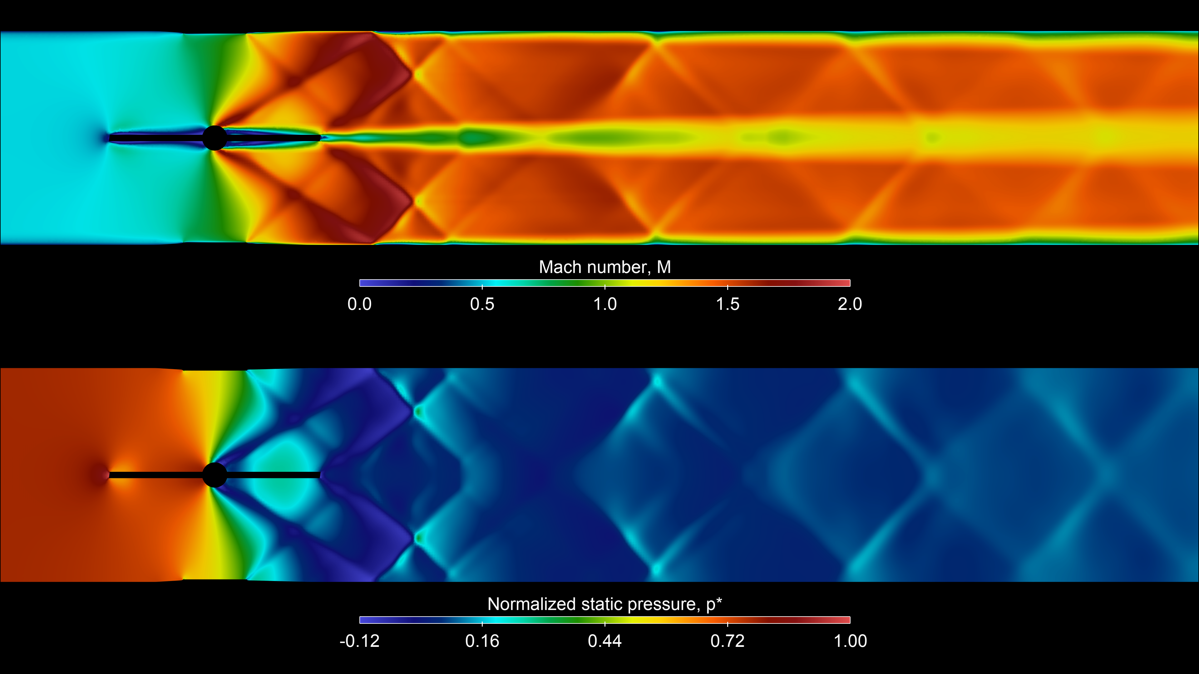
The selected image shows a generic geometry and flow field. Validation and delivered industrial curves belong to the professional project; they are not measurements of this public example.
01 / DEFINE A USEFUL COMPARISON
A valve does not have one mass-flow value. Its opening and upstream/downstream conditions define the operating point.
The professional campaign combined pressure conditions with valve openings, checked the model where test data existed, and delivered curves for subsequent engineering use. Consistent pressure references and reporting locations made those comparisons meaningful.
The public Mach and pressure panels show why that matrix needs compressible CFD: the restriction accelerates the gas, changes its density and creates downstream expansion and compression structures.
The private Python drivers automate one configurable mesh/setup workflow; they do not generate an automatic multi-angle geometry sweep.
02 / FLOW INTERPRETATION
The two panels describe the same type of engineering question from different quantities: where the gas accelerates and how static pressure varies through the restriction.
The upper panel shows acceleration around the plate and a downstream jet with local supersonic regions. The compression and expansion pattern is a reason to resolve density and energy rather than assume constant-density flow.
The lower panel relates local static pressure to inlet and outlet reference values. These visualization references differ from the solver’s inlet total-pressure condition. Negative normalized values indicate pressure below the chosen outlet reference; they do not imply negative absolute pressure.
Normalization makes the pattern readable without disclosing an industrial pressure condition. It does not establish that different operating points have the same flow behavior.
For characterization, combine the field view with mass flow, pressure definitions, valve opening and convergence evidence for each operating point. This image alone does not demonstrate validation or an optimized component.
03 / REUSABLE WORKFLOW
Two Python drivers keep model configuration readable and make repeated setup less dependent on manual Fluent sessions.
Watertight Geometry with specified surface sizes, smooth-transition boundary layers and poly-hexcore volume meshing. The WFT reference records the selected settings.
Steady density-based implicit solver, energy, ideal-gas air, Sutherland viscosity and k–ω SST. Named expressions define pressure conditions; measurement planes support the reports.
The setup driver creates surfaces and base reports before compound expressions. Separate setup, run and all modes preserve the documented initialization and iteration procedure.
Earlier development notes record matching reference/rebuilt mesh counts and individual solver API checks. Equal counts do not establish mesh independence, and a complete converged 2,500-iteration run was not demonstrated. No solver was run for this publication.
CAD and meshes are excluded and must be supplied locally. The documentation identifies checks still needed for operating pressure, measurement-plane placement and report validity. The cd_a expression is an equivalent area in m², not a dimensionless discharge coefficient or a general compressible-flow correction.
04 / TRANSFERABLE SKILLS
The same analysis methods can support valves, restrictions, air paths and gas-delivery systems, with model choices and validation adapted to each application.
Relate acceleration, density change and pressure recovery to the quantities an engineer needs.
Flow interpretation ↑Establish the method on a measurable component, then use a controlled operating matrix to extend characterization to larger equipment.
Study context ↑Build reusable mesh and setup drivers, with explicit report dependencies and local prerequisites.
Workflow ↑Implementation files and detailed configurations are maintained privately. This page presents the engineering approach and selected evidence.
© 2026 Alberto Brambila Solórzano. All rights reserved.