The research question
In pulsatile vascular flow, viscosity, turbulence assumptions and wall motion can change the quantities being interpreted. Their effects need to be separated.
DOCTORAL RESEARCH · UNAM · THERMOFLUIDS · 2025
Which predictions change when blood rheology, turbulence or wall motion are modeled differently? My doctoral work examined those choices and their effects on flow and particle transport.
MY WORKDeveloped CFD methodology, software and analysis; investigated model assumptions, performed validation and contributed original research writing alongside collaborators. Clinical resources and research support were collaborative.
DOCTORAL RESEARCH / MODEL CHOICE AND VALIDATION
In pulsatile vascular flow, viscosity, turbulence assumptions and wall motion can change the quantities being interpreted. Their effects need to be separated.
I developed and assessed CFD methods for rheology, fluid–structure interaction and particle transport, supported by benchmark and sensitivity checks.
Separate comparisons show how model choices affect flow, wall-shear measures and transport. Together they demonstrate how to assess a multiphysics model rather than rely on one attractive flow field.
These are related doctoral studies with their own geometries and checks, not a single validated clinical prediction. The same modeling and verification skills transfer to other coupled internal-flow problems.
01 / MODEL FIDELITY
Geometry, viscosity law and flow-model assumptions interact. The research compared them through defined outputs instead of treating increased model complexity as a guarantee of a better answer.
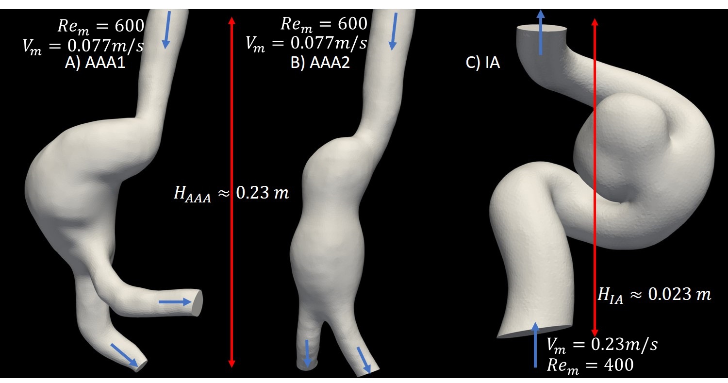
Image-based domain preparation, inlet/outlet definition and near-wall meshing established the computational regions. The model-comparison study imposed pulsatile inflow with a 0.75 s period, then examined constitutive and laminar/k–ε assumptions.
Three different geometries made it possible to ask whether a conclusion was a feature of the chosen model or of the particular flow domain.
The transferable task: make a modeling choice defensible by holding the comparison conditions clear and measuring its effect on an engineering output.
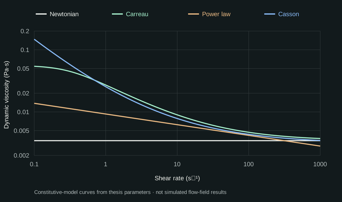
A constant Newtonian viscosity is a baseline. Carreau, power-law and Casson descriptions give different low-shear behavior—precisely where recirculation can make a constitutive assumption important.
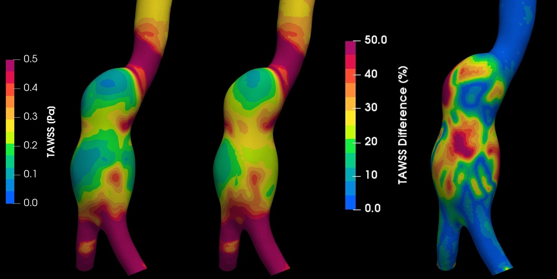
The thesis reports mean TAWSS differences between Carreau and Newtonian cases of 19%, 16% and 3% for AAA1, AAA2 and IA. The small difference in one geometry cannot justify a universal Newtonian approximation.
The useful conclusion is a sensitivity assessment: decide whether the viscosity model matters for the flow region and output being used.
TAWSS is cycle-averaged wall-shear magnitude, in Pa. OSI measures shear-direction oscillation. They answer different questions; a similar mean shear level can coexist with a changed directional history.
Extracting, averaging and interpreting these outputs is part of the work—not just selecting a solver option.
Newtonian: μ = 0.00345 Pa·s. Carreau: μ = μ∞ + (μ₀ − μ∞)[1 + (λγ̇)²](n−1)/2, with μ₀ = 0.056 Pa·s, μ∞ = 0.00345 Pa·s, λ = 3.313 s and n = 0.3568.
Power law: μ = Kγ̇n−1, K = 0.009267 Pa·sⁿ and n = 0.828. Casson: μ = [√(τc/γ̇) + √m]², with m = 0.0031 Pa·s and τc = 0.01081 Pa. The displayed 0.1–1000 s⁻¹ interval illustrates these laws; it is not a measured shear-rate range for every case.
The work compared laminar and standard k–ε descriptions and examined behavior across pulsatile cycles. Later-cycle OSI patterns changed more in the aortic comparison than in the selected intracranial geometry.
This demonstrates turbulence-model assessment and time-dependent interpretation. Recirculation or cycle variation alone does not establish turbulent flow; these were not DNS or LES calculations.
The animation below is a separate, idealized sidewall-sac visualization. Following the vectors helps explain inflow, local rotation and exchange with a recirculating region before reading more abstract wall indices.
Its vectors represent the velocity field, not particle trajectories or proof of turbulence.
02 / FLUID–STRUCTURE INTERACTION
A deformable boundary introduces an additional feedback: fluid forces change the wall, and the moving wall changes the flow domain.
The formulation used a linear isotropic elastic wall and an arbitrary Lagrangian–Eulerian description for the fluid mesh. The surviving solids4Foam benchmark configuration selects partitioned IQN-ILS coupling.
This requires attention to interface transfer, mesh motion and convergence in addition to the fluid solution itself.
The selected aortic rigid/elastic comparison reports differences of 23% in diastolic WSS, 19% in OSI and 43% in GON. GON describes temporal cancellation of the wall-shear-gradient vector.
The importance of wall motion therefore depends on the output. Similar broad flow patterns do not establish agreement in oscillatory or gradient-sensitive quantities.
Transfer: coupling fluid loads, structural deformation and mesh motion is the same class of numerical task encountered in compliant flow passages, flexible components and other fluid-loaded structures. Those applications are skill transfers, not additional projects claimed here.
03 / VERIFICATION AND VALIDATION
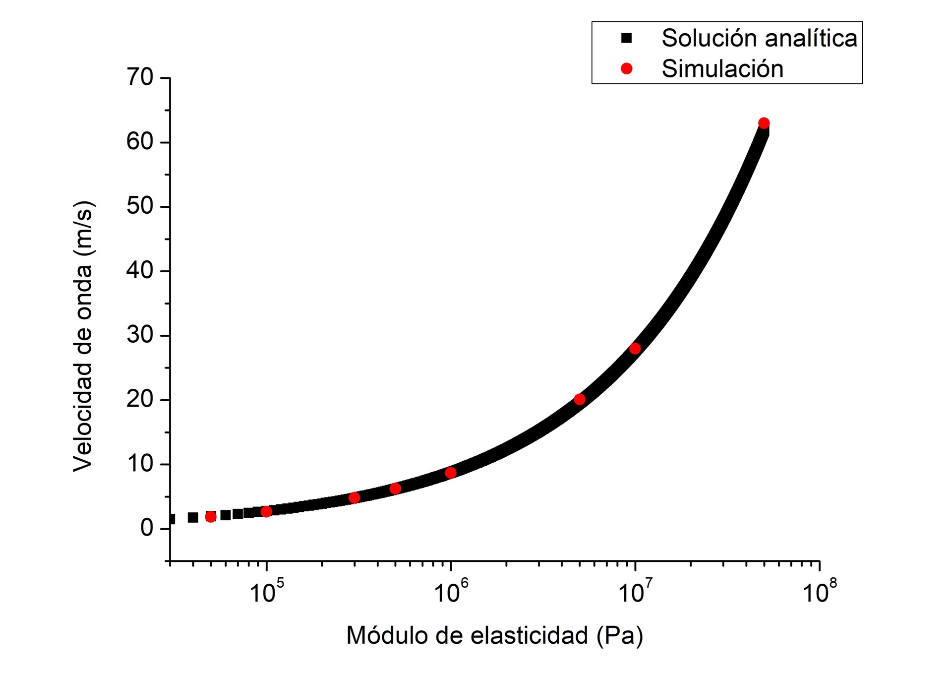
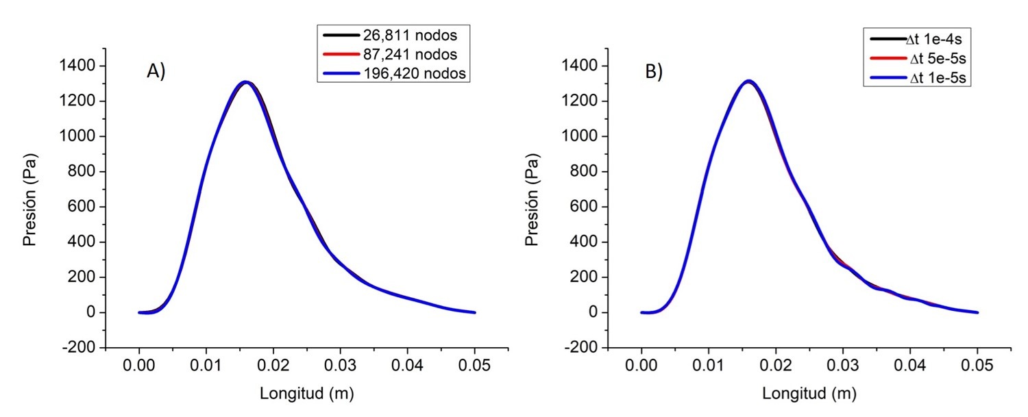
An elastic-tube pressure wave isolates the fluid/solid feedback before complex geometry is introduced. The benchmark connects animation, analytical prediction and numerical sensitivity.
The thesis benchmark uses a 1333 Pa pulse lasting 0.003 s. The analytical relation combines fluid compressibility and wall compliance, giving a reference for the numerical pressure-wave speed.
The reported maximum analytical/numerical discrepancy is 6%. It is meaningful because the compared quantity, the reference and the tested family are defined.
This verifies a coupled numerical response. It does not validate anatomical material properties or a clinical outcome.
For the elastic tube, mesh and time-step comparisons examined the pressure profile. The thesis reports differences up to approximately 3% for mesh and 2% for time step. The full plots make the sensitivity visible instead of reducing validation to a badge.
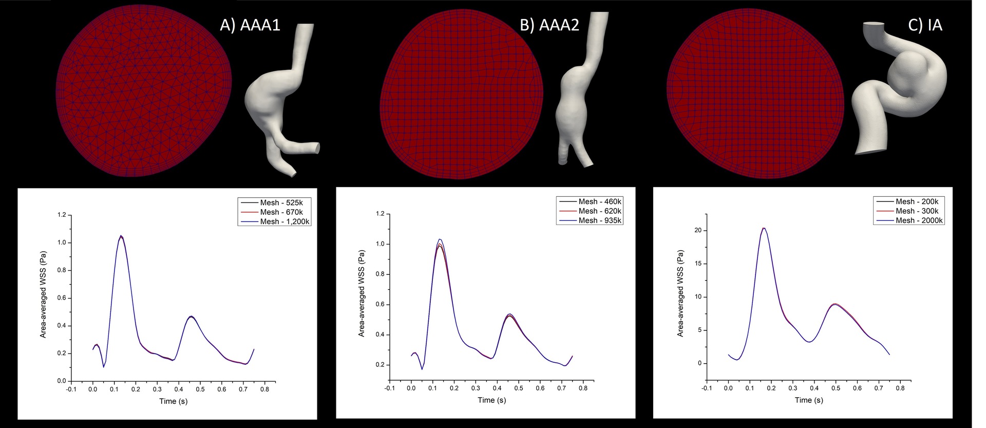
The separate aneurysm meshes were assessed through surface-averaged WSS histories over a pulsatile cycle. Near-wall resolution and the time-dependent output are shown together, linking meshing decisions to the quantity eventually interpreted.
04 / LAGRANGIAN TRANSPORT
Particle tracking adds a different question: how injected material moves through the unsteady field and exchanges with recirculating regions.
A surviving DPMFoam setup specifies one-way Lagrangian tracking, inlet injection, 5 μm particles, sphere drag and rebound at walls. One-way coupling means particles respond to the carrier flow without feeding forces back into it.
Injection, particle properties and wall interaction are physical modeling choices. They determine what the trajectory calculation can represent.
Age is elapsed time since injection. It is different from RRT, a wall-shear-derived index, and from a residence-time distribution calculated from trajectories.
The work demonstrates dispersed-phase configuration and transient transport visualization. Quantitative trapping or residence statistics require the corresponding trajectory data and run definition.
Transfer: Lagrangian injection, drag and wall-interaction modeling are relevant to dispersed-material transport in internal flows. Particle size, forces and coupling assumptions would be reassessed for each new application.
WHAT THIS WORK BRINGS TO ANOTHER PROJECT
The application was biomedical flow. The transferable experience is the ability to construct, compare and assess physical models and their numerical implementation.
Coupled fluid traction, elastic deformation and moving-mesh response; checked pressure-wave propagation against an analytical reference.
Transfer: Compliant channels, flexible fluid-loaded components and coupled multiphysics simulation.
See the engineering evidence ↑Compared four viscosity laws and quantified geometry-dependent changes in cycle-averaged shear.
Transfer: Assessing shear-dependent fluids in process equipment and complex internal passages.
See the engineering evidence ↑Compared laminar/k–ε assumptions and interpreted cycle-dependent quantities without equating vortices with resolved turbulence.
Transfer: Choosing and evaluating flow models for transient recirculating systems.
See the engineering evidence ↑Configured injection, particle properties, drag and wall interaction; interpreted age-colored trajectories.
Transfer: Dispersed-phase transport studies with application-specific force and coupling assumptions.
See the engineering evidence ↑Used analytical comparison, pressure-profile refinement and time-dependent WSS mesh comparisons.
Transfer: Building confidence in a simulation before using its outputs in a design or research conclusion.
See the engineering evidence ↑Prepared complex image-derived domains and extracted defined surface/volume metrics across geometries.
Transfer: Complex-domain preparation, meaningful averaging and technical communication of CFD results.
See the engineering evidence ↑These chapters connect related study families, not one complete factorial campaign. Percentages are thesis-reported comparisons; underlying normalization has not been independently recomputed here. The later intracranial cohort is documented in the research records, with overlapping distributions and data-accounting limits; no clinical predictor is claimed.
Wall motion is qualitative without a verified display multiplier. Current dictionaries, thesis tables and publication settings represent different research versions. A complete executable reproduction has not been established; no new CFD runs were performed for this website.
Research figures and animations: Alberto Brambila Solórzano and collaborators, UNAM. The related Bioengineering 2023 article is CC BY 4.0; that license is not a blanket license for other research assets. Original clinical records and anatomy files are not distributed here.
Related publication: Blood rheology and turbulence model comparison, Bioengineering (2023) ↗.
Implementation files and detailed configurations are maintained privately. This page presents the engineering approach and selected evidence.
© 2026 Alberto Brambila Solórzano. All rights reserved.