The problem
Air carried by the liquid needs a path to separate. Changes that improve separation also need to be assessed for their effect on flow resistance.
MULTIPHASE FLOW / GENERIC DEMONSTRATOR
How does the flow path affect air separation and pressure loss? This generic demonstration illustrates the VOF modeling and design-comparison methods I used in professional degassing work.
Alberto Brambila, PhD
Multiphase modeling · Net-flux analysis
CAD-to-mesh and solver-setup automation
PROFESSIONAL EXPERIENCE / AIR SEPARATION
Air carried by the liquid needs a path to separate. Changes that improve separation also need to be assessed for their effect on flow resistance.
I led VOF simulations and worked with mechanical designers to compare geometry variants, track air transport and assess pressure loss.
The comparisons explained why some flow paths separated air more effectively and guided the selection of a design for physical testing.
Both the professional study and this generic demonstration use VOF. The geometry and results shown here belong only to the demonstration; its 78.2% routing value is not an industrial performance result.
01 / THE DESIGN LEVER
A bubble can follow the liquid back into the circuit or rise into the reservoir. The useful design change alters that competition without adding excessive flow resistance.
Local liquid velocity competes with bubble rise. Slowing or redirecting the flow can give buoyancy more time to act; bubble size and the surrounding flow affect the resulting trajectory.
The design question was therefore not simply “add a baffle,” but where to change the flow and what pressure penalty that introduced.
The VOF demonstration resolves air–liquid interfaces moving through the junction and interacting with the upper surface. Gravity, surface tension and turbulent liquid flow shape that motion.
The next figures turn the visible flow path into a defined transport measurement, then show how the same comparison format can support design screening.
02 / CONNECT MOTION WITH A MEASUREMENT
The demo reaches 78.2% cumulative net air routing to the reservoir plane at 15 s. This is a sensor-defined CFD transport ratio for the displayed demonstration, not measured external removal efficiency.
Design comparison benefits from two views: a history that shows transport delay and accumulation, and a common endpoint that makes the chosen metric easy to compare.
This is the type of comparative analysis used in Alberto’s professional degassing work. Here, the blue series is the simplified geometry’s CFD result; the other 15 variants are illustrative examples, not the original industrial results.
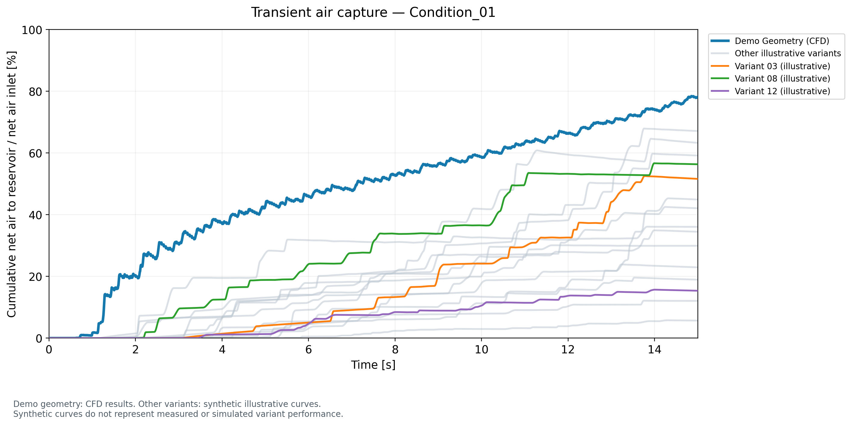
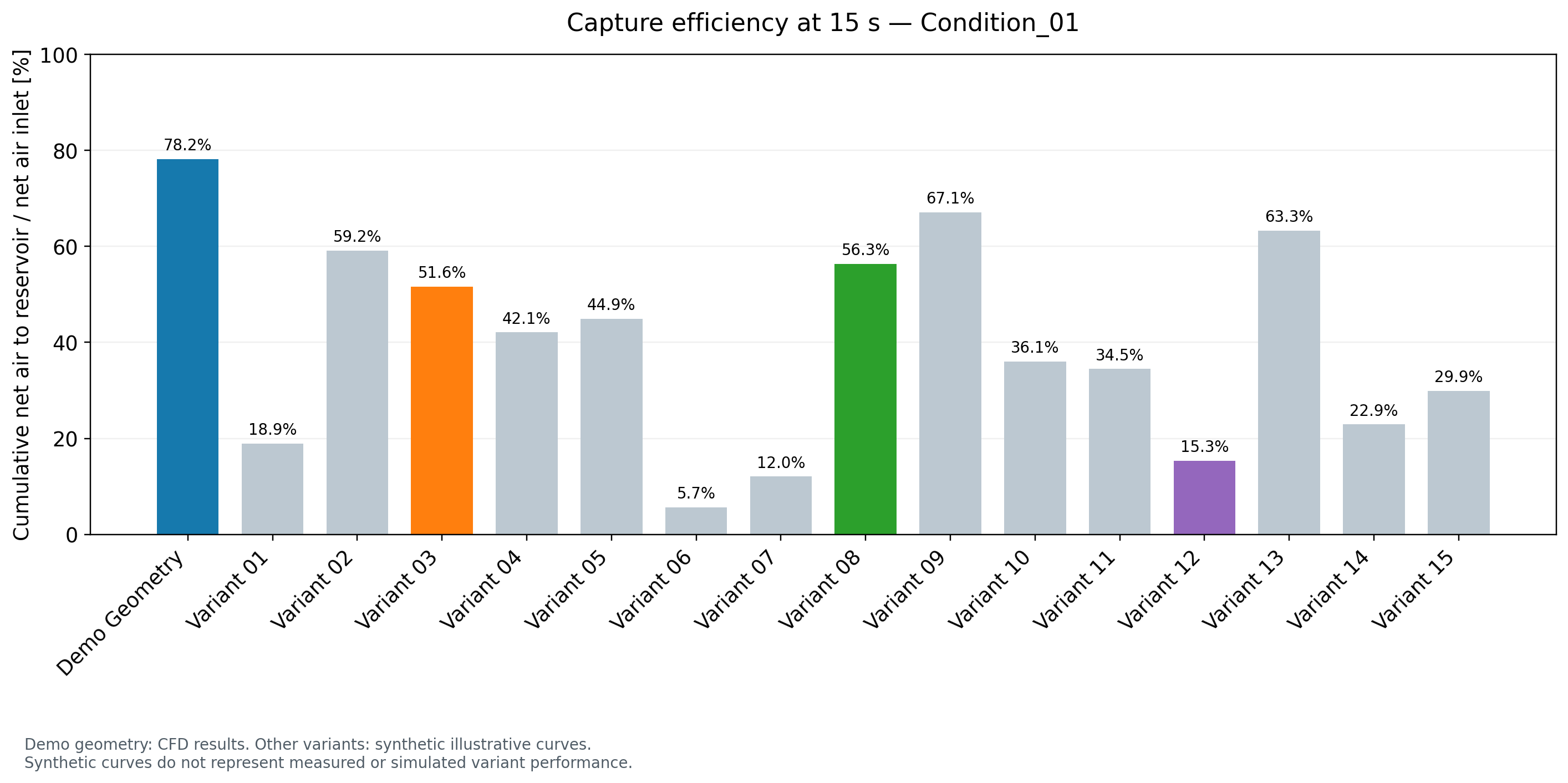
The calculation integrates the signed air mass flow at the reservoir plane and divides by integrated inlet air mass over the same 0–15 s window. The reservoir signal is reversed to match the chosen positive transport direction.
η(T) = 100 × M_air,reservoir(T) / M_air,inlet(T)
The reservoir sensor is an internal plane. The saved boundary assignments restrict air exit, so this ratio describes net internal routing rather than proving permanent capture or zero downstream carryover.
The supplied history independently gives 4.8661 × 10⁻⁵ kg of net injected air and 3.8064 × 10⁻⁵ kg routed across the reservoir plane.
Engineering decision: use the transient history to understand transport delays, then assess pressure loss, carryover, conservation and numerical sensitivity before choosing a design. The demo does not establish a validated optimum.
03 / MAKE THE WORKFLOW REUSABLE
The automation work addresses a practical CFD failure mode: a regenerated mesh can acquire boundary types and IDs that differ from those used to define the solver model.
Locate the generic CAD by extension; apply configurable surface sizing, three prism layers and poly-hexcore volume meshing.
Read the local reference case, replace the mesh by zone name and retain boundary types, expressions, reports and surfaces.
Integrate oriented phase fluxes over the same time interval; connect the calculated quantity to the physical question.
Separate configurable meshing and setup drivers make the workflow reusable. The implementation stays private; the diagram above explains the modeling and verification sequence.
WHAT THIS EXPERIENCE BRINGS TO YOUR TEAM
The same skills support cooling loops, filling operations, phase separators and other internal-flow systems. The model assumptions and validation plan must follow the new application.
Translate air ingestion, gravity and interfacial physics into a tractable transient model.
Transfer: liquid-management and gas–liquid transport problems.
See the physical choices ↑Compare air routing over the same operating window, then weigh separation against pressure loss before selecting a prototype.
Transfer: consistent comparison, conservation checks and evidence-based decisions.
See the calculation ↑Turn repeated mesh and setup work into configurable Python drivers, while checking zone assignments and report definitions.
Transfer: repeatable virtual prototypes and fewer manual setup mistakes.
See the workflow ↑This generic/simplified geometry is a public demonstration. Broader professional experience includes iterative degassing design analysis and collaboration with mechanical design and test teams; those industrial outcomes are separate from the results shown here.
This demonstration uses transient VOF. Validation from the professional project does not validate this separate model. No new CFD solve, experimental comparison or mesh/time sensitivity campaign was performed for publication.
Animation timing assumes uniformly spaced original frames. The assigned liquid uses water-like properties, despite a separate unused coolant material in the reference. Original private metadata, cases, meshes and Fluent outputs are excluded.
Implementation files and detailed configurations are maintained privately. This page presents the engineering approach and selected evidence.
© 2026 Alberto Brambila Solórzano. All rights reserved.